Measuring geodetic distance calculation performance
Introduction
Earth is not flat, although, on many occasions, I wished it was. Geometric calculations such as finding the distance between two points or the closest distance between a line and a point are simple on flat surfaces, but things become much more complex on a curved surface. Instead of geometric, these operations are called geodetic calculations.
The need for accurate geodetic computations
On a traditional Mercator projection map, such as the one shown in Figure 1, transatlantic navigation seems simple: just measure the angle between your current location and the target, take a compass heading and steam on. The red line on Figure 1 shows the rhumb line between Southampton and Miami. Indeed, due to its simplicity, that still is a commonly used navigation method. At this day, though, it’s not really smart. If you draw the same route on a different projection, such as the orthographic projection in Figure 2, it becomes apparent that the red line is not the shortest one by any measure.
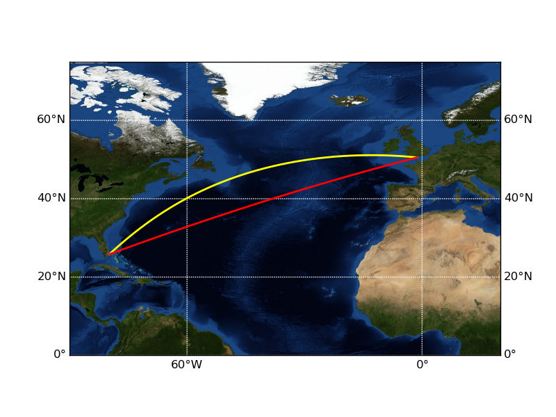
Figure 1: Voyage from Southampton to New York, in Mercator projection.
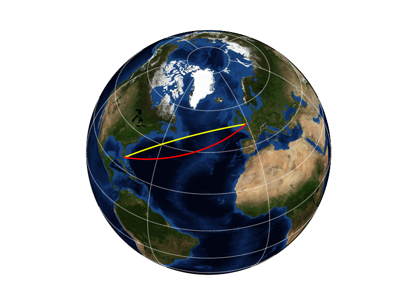
Figure 2: Voyage from Southampton to New York, in orthogonal projection.
The shortest route between two points on a spherical surface is along the great circle shown on Figure 1 and Figure 2 by the yellow lines. As indicated by the curved line on the Mercator projection, the compass heading varies along the great circle route, but nevertheless, that is the optimal route to take. The rhumb line distance in our example is 3932 nautical miles (nmi), while the great circle distance is 3804 nmi, a difference of 3.4%. On a suitable leg, the distance difference might be considerably higher.
Great circle calculations on a spherical surface are actually not that complicated. Analytical (closed-form) solutions exist for most problems [1], and although the formula are more complex than their counterparts in planar geometry, the added complexity is insignificant for modern computers.
Unfortunately, our problems don’t end here. Not only is the Earth round, but it isn’t round enough. Due to Earth’s rotation, it is slightly flattened at the poles: the diameter at the poles is approximately 42 km shorter than the diameter at the equator. Hence, the Earth’s shape is commonly approximated as an ellipsoid. The measured flattening is quite small, 1/298.25, but still is sufficient to cause errors of up to 0.55% (typically less than 0.3%) if spherical assumption is used. Since the fuel savings provided by Eniram‘s products are in the order of 2–6%, we definitely don’t have a sufficient margin to allow that kind of errors in our calculations.
As a practical example, on the Southampton–Miami voyage, the distance measured on a WGS84 geoid is 6.6 nmi larger than on a spherical surface, an error of 0.17%. This error corresponds to 20–30 minutes of increased travel time, or close to 1500–2000 USD of fuel costs on a big ship – certainly nothing to sneer at.
On ellipsoid surfaces, the great circle calculations get really complex. No closed-form formulas exist for most of the problems, and numerical solutions must be used. Of course, excellent libraries performing all the required calculations for different ellipsoids exist, e.g. proj.4 and its Python bindings, pyproj. However, the numerical formulas are much slower than the analytical ones. Many common operations require a massive amount of geodetic calculations. For example, we might have a voyage consisting of 20 waypoints. To simply find out the distance remaining on the voyage, we need to project the ship’s actual location on each of the 19 sublegs. On an ellipsoid surface, each projection calculation includes an optimization loop and requires perhaps 10–12 distance calculations, or a total of 190–228 calculations. If this is performed for every point on a historical track of, say, 40,000 points, the time required by the projection calculations may become a genuine issue even with highly optimized libraries such as proj.4.
Algorithm execution times
To illustrate the speed difference of different algorithms, I ran a piece of code projecting 1000 points on a line with three different algorithms: analytic (spherical projection), numeric (with pyproj) and hybrid. The analytic algorithm uses closed-form formulas presented in [1]. The numeric and hybrid algorithms find a numeric solution by optimizing the geometry shown in Figure 3. Distance \(y\) from \(P\) to \(P'\) is calculated for different values of \(d\). When \(y\) is minimized, we have a solution for \(P'\). The difference between the latter two algorithms is that the numeric one uses the GPS standard WGS84 [2] projection everywhere, while the hybrid algorithm calculates the \(d\) and \(y\) distances using spherical projection.

Figure 3: Numerical approximation of point projection.
Figure 4 shows the test results. Even though the projection was run in a scalar fashion (looping through the points) and therefore there was a significant execution overhead, the analytic solution is almost an order of magnitude faster than the numeric ones. There is a small but rather insignificant gain acquired in the hybrid version.

Figure 4: Test run results.
Discussion
The test in the previous section was for one segment only. A typical voyage contains multiple waypoints, and finding our location on the voyage requires at least one projection calculation for each segment. Therefore, the algorithm selection becomes crucial for our optimization performance. In practice, we need to perform the projection calculations with the spherical formulas, and then re-calculate the distance d using the ellipsoid algorithms provided by pyproj. This provides us a reasonable accuracy and good computational performance. This is one of the examples in which careful algorithm selection is crucial. Without thinking, we could either have a really fast implementation and insufficient accuracy, or a really accurate implementation running with a glacial speed. By designing our implementation carefully, we are able to get the best of the both worlds.
The calculations above leave much room for improvement regarding performance. Direct Numpy implementation of the analytic spherical formula, even when vectorized, requires multiple temporary arrays to store the intermediate results. The ellipsoid versions do not run vectorized at all, but need to be looped instead. In the next blog post, we will pluck some low-hanging performance fruit by re-implementing our geodesy calculations in Cython.
| [1] | (1, 2) See e.g. http://www.movable-type.co.uk/scripts/latlong.html |
| [2] | http://en.wikipedia.org/wiki/World_Geodetic_System |
Matti Airas is a senior research developer at Eniram. He is a member of Eniram’s Algorithm Development team, responsible for developing the Python based backbone of Eniram’s products. When not at work, he enjoys performing experiments on his Spanish Water Dog, sailing, creating weird items with his 3D printer, and fiddling with radio-controlled devices.