Implementing a geospatial database with Python
Introduction
When we model and optimize energy consumption of ships we typically deal with large geospatial and temporal datasets. For instance, most commonly we need to find the values of various meteorological forecasts along the whole of a vessel’s route. Such a route may span across oceans and can take many days for a ship to complete. Also, we would like the data to be delivered on-board as fast as possible. Suffice it to say, our production environment needs at least robust and reliable storage of the data and effective access to it.
We have decided to use a somewhat custom approach in our databases. The base of our databases are NetCDF4 files, from which data can be extracted efficiently. Initially we thought that there should exist standard tools that would fit to our problems, but we were surprised and disappointed to find out that this is not the case. The biggest caveat of existing tools seems to be that temporal dimension isn’t at level with spatial ones. For us, the treatment of time should be in many ways analogous to the treatment of spatial dimensions.
In this post, we will show an example database implementation that uses NetCDF4 files to store the data. This highlights some of the problems we have encountered and design choices we have made.
Before diving into the example, we will spend a little time explaining the terminology and our data. If you just one want to see the code and skip all the rambling, go to Basic elements of our database solution. After the code example we will discuss briefly other tools we have investigated.
Short introduction to GIS concepts
Geospatial libraries usually use the terminology of GIS (Geographic information systems), and we will also use it in this post. In this section two basic objects are discussed: vector and raster. Examples of the objects can be found in visualizations of Our data.
We are mostly concerned with raster data in our applications. A raster object can contain one or more matrices of equal size, where each cell of a matrix corresponds to a patch, or a pixel, in some geographical location. The cell value can then be a physical quantity like temperature, humidity, or elevation, at the corresponding location.
In our data raster pixel locations are expressed in equally spaced latitude and longitude values. These latitude and longitude values further correpond to a certain model of Earth, in our case WGS84.
A raster can contain multiple bands, i.e., data matrices. For instance, if a raster only expresses a color value in each pixel, there can be three bands, red, green, and blue. Another example is our sea current data, which contains north and east components. The two components could be expressed as their own bands. However, in our databases we have defined raster bands to express different time instances.
Another key concept of GIS is an object called vector. Vector is referenced to fixed geographic points but not to pixels. Vector can also contain attributes to each point. Typical examples of vector features are roads, rivers, coastal lines, or boundaries of countries. In our case the route of a ship can be considered as a vector feature.
Our data
This post focuses on forecast data of globally gridded simulation values that describe different meteorological variables at sea.
Our data is typically downloaded on-board a ship at fixed time intervals or when a ship visits a port. It is only practical to download that spatio-temporal subset of meteorological data which is relevant for the ship’s voyage.
One use case for our data is speed optimization in which the latitude and longitude points of a route are known but exact time points are variables in the optimization. In other applications we may also wish to optimize the route. In this case also latitude and longitude points are not fixed when the data is downloaded. When we download data from a database, there needs to be enough of it to cover different use cases.
An example dataset is described below in three figures. These visualize forecast data of one variable at different levels. Figure 1 shows a close-up on what raster data looks like, and how spatial points between pixel locations can be approximated with linear interpolation.
Figure 1: Only a few pixels from a relative humidity raster. The right plot shows linearly interpolated pixel values. A point of interest ‘x’ is plotted to highlight the problem of estimating a value in between pixel center points.
Figure 2 views the raster data globally for one time instance. In the figure a possible ship route is visualized to describe the extent of data that may need to be extracted from the raster.
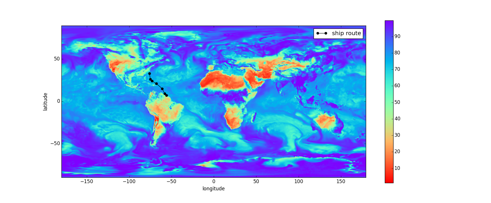
Figure 2: Relative humidity raster band for one time instance.
Figure 3 visualizes the two time dimensions that we have in our data. The first time dimension tells us what time instance a raster applies to. The second time dimension is the release time of a forecast. Usually there is overlap between different forecast releases and ideally we would like to use the newest available forecasts for each route time point.
The time axis also contains example route points. When these points are not exactly aligned with forecast time instances, we need to interpolate to get proper estimates for forecasts.
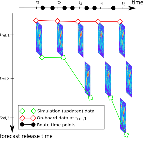
Figure 3: Many relative humidity rasters with bands corresponding to different time instances. Red and green lines both denote possible collections of data matrices used for our optimizations. First, red line denotes the data that is obtained in real-time at the start of the route. Green line then denotes data where we have updated the last three matrices to more recent forecasts, which were not available at the start of the route.
Basic elements of our database solution
In this section we show by a small example how we have built our databases on NetCDF4 files which have been mounted to a local filesystem. The following code is far from production ready, but it should highlight some of the design choices we have made.
The following code moderately exploits NumPy, Scipy, and Pandas. If you are unfamiliar with these numerical tools, you probably have to consult their documentation to understand the details.
In this example we use only one NetCDF4 file for air temperature. If you wish to run the code, you have to include this file in your current working directory. This particular data file isn’t used in our products, but the structure resembles that of our actual data.
We start the example by importing the numerical tools and a class that can open NetCDF4 files for reading:
import numpy as np
import pandas as pd
from scipy.interpolate import interpn
from netCDF4 import Dataset
Then let’s define what the final output will be like. We want to create a database class from which we can request forecast data for a ship’s route. We would like the database to provide us with regularly gridded data so that we can then easily use SciPy’s interpolator estimate values for the route. Expressed in code:
if __name__ == '__main__':

    # "random" coordinates
    lat = np.r_[30., 30.2, 30.4, 30.9]
    lon = np.r_[150.1, 150.2, 151.5, 152.]
    # hours since 1800-01-01 00:00:0.0
    time = np.r_[1884649., 1884655., 1884660., 1884670.]
    route = np.c_[time, lat, lon]

    # Example data contains variable 'air' for air temperature
    db = Database()
    clipped_data, axis_points = db.clip_data(route, 'air')

    # Flip latitude axis because that is not ascending in our data
    axis_points[1].sort()
    clipped_data = clipped_data[:,::-1,:]

    interpolated_values = interpn(axis_points, clipped_data, route)
Above, clipping the data means that we extract a “cube” of raster points so that all the three dimensional route points are contained within the cube’s outermost cells. axis_points is then a tuple of three arrays which contain time, latitude and longitude values that correspond to the cells inside the cube.
Now we can continue implementing the actual database class:
class Database(object):

    def clip_data(self, route, varname):
        """Read subsets of data raster data to cover all requested points

        """
        # Vectors that define the route
        time, lat, lon = route.T
        # Open required files and group time instances according to them
        datasets = self._get_datasets(time, varname)
        # Loop over files and time vectors corresponding to them
        for ds, t in datasets:
            clipped, axis_points = _clip_one_dataset(ds, varname, lat, lon, t)
            ds.close()

        # We should concatenate all clipped data according to time axis.
        # We should also concatenate all time axis axis_points.
        # Latitude and longitude axis_points are the same in all.

        return clipped, axis_points

    def _get_datasets(self, time, varname):
        """Find files from which to get variable for requested times

        All database files contain different time instances.

        """
        # Return only one example data set, which contains all
        # times that can requested
        return [(Dataset('air.2015.nc'), time)]
Nothing complex there. The idea in clip_data is that the database instance first looks at the requested times and then opens corresponding NetCDF4 files. Then the vector for requested times is divided according to the opened files.
Now the index of database files is completely missing, as well as the logic that decides which files to open. These are minor implementation details which we have chosen to skip here. Instead, we just open one file in the current working directory. In reality the different clipped data should also be concatenated together, but that is another detail which we skip for simplicity.
The function that hasn’t yet been defined, _clip_one_dataset, accesses only the needed values in NetCDF4 files and returns those as its first return value. The second return values contains axis values which correspond to the returned point values. In this example the function is defined as follows:
def _clip_one_dataset(dataset, varname, lat, lon, time):
    """Find all NetCDF4 file values that cover the requested axis values

    """
    def get_required(axis_name, requested_values):
        axis = pd.Series(dataset.variables[axis_name][:])
        axis_step = abs(axis.iloc[1] - axis.iloc[0])
        return axis[(axis > requested_values.min() - axis_step)
                    & (axis < requested_values.max() + axis_step)]

    required_lat = get_required('lat', lat)
    required_lon = get_required('lon', lon)
    required_time = get_required('time', time)

    clipped = dataset.variables[varname][required_time.index,
                                         0,  # height axis
                                         required_lat.index,
                                         required_lon.index]

    axis_points = (required_time.values,
                   required_lat.values,
                   required_lon.values)

    return clipped, axis_points
The function first defines a smaller function which finds sub-sets of axes with that surround requested axis values. After the sub-sets are obtained, the corresponding forecast values are extract using the Dataset API. Here there is an extra axis variables, height, which was also contained in this example data.
And that’s it! There is our rudimentary database implementation.
Discussion: another way to build similar functionality
In this post we have discussed building a simple custom geospatial database on top of NetCDF4 files. Most of the discussion has been around only one aspect of the database: how data can be extracted from files and returned through a simple Python API. In real-life many other problems have to be solved by our database: indexing of data files for effective access, different query functionalities, error handling, different APIs (e.g., REST over web), and so forth.
Any unnecessary custom building blocks are worrying as they bring about maintenance burden, and their development is costly at any rate. One existing database that we have considered for our data is PostgreSQL with PostGIS extension that supports all kinds of geospatial data. PostGIS project is part of OSGeo foundation which provides all kinds of tools for Geospatial data processing and analysis. Some other OSGeo libraries are already incorporated into our codebase.
PostGIS defines a raster data type in which our forecast data could be expressed. Basically, PostGIS divides a raster into tiles that describe different part of a globe and puts those tiles into one database table. Rasters can also be imported conveniently into the database with another OSGeo library, GDAL (which also provides nice Python bindings).
However, there doesn’t seem to be a standard way of representing temporal rasters in PostGIS. For instance, with the GDAL import tool temporal metadata is completely ignored. Thus it would require some additional work to maintain the temporal metadata in the database. Some work would also go into maintaining a master table that cross-references to tables of different variables and forecast release times. Also, we would still have to build somewhere the logic of choosing the rasters with right time instances and forecast release times.
Admittedly, PostGIS would provide a suite of other functionalities that might be convenient in the future. However, so far the benefits haven’t outweighted the flexibility provided by our custom database implementation.
Jarno Saarimäki is a senior research engineer in Algorithm Development team at Eniram. Jarno’s educational background is in numerical analysis and geoscience but he is also an avid programmer. Outside of work he enjoys hiking in nature, reading historical books, and playing board games.